Gaussian mixture models assume that the patterns ![]() origin from a probability density
p(
origin from a probability density
p(![]() ) (Bishop, 1995). This density is a linear combination of Gaussian functions
p(
) (Bishop, 1995). This density is a linear combination of Gaussian functions
p(![]() | j),
| j),
The density
p(![]() ) is a weighted sum of the local densities
p(
) is a weighted sum of the local densities
p(![]() | j),
| j),
| p( |
(2.17) |
The goal of the mixture model is to find the unknown parameters ![]() ,
, ![]() , and the priors P(j) for each unit j such that the likelihood,
L =
, and the priors P(j) for each unit j such that the likelihood,
L = ![]() p(
p(![]() ), to obtain the distribution
{
), to obtain the distribution
{![]() } given the density
p(
} given the density
p(![]() ) is maximal (Bishop, 1995). To solve this optimization problem it is common to use a variant of the expectation maximization algorithm (Bishop, 1995). It consists of two steps with iterate until convergence is reached. In the expectation step, the soft-assignment
P(j|
) is maximal (Bishop, 1995). To solve this optimization problem it is common to use a variant of the expectation maximization algorithm (Bishop, 1995). It consists of two steps with iterate until convergence is reached. In the expectation step, the soft-assignment
P(j|![]() ) for all j and i is computed based on a given estimate of the parameters
) for all j and i is computed based on a given estimate of the parameters ![]() ,
, ![]() , and P(j).
P(j|
, and P(j).
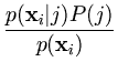
P(j|![]() ) is called posterior probability. It is computed using Bayes' theorem (see appendix A.1),
) is called posterior probability. It is computed using Bayes' theorem (see appendix A.1),
In the maximization step, the Gaussian's parameters ![]() ,
, ![]() , and P(j) that maximize the likelihood given all
P(j|
, and P(j) that maximize the likelihood given all
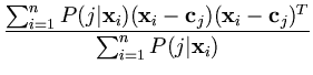
P(j|![]() ) can be directly computed (Bishop, 1995). The result is that the center
) can be directly computed (Bishop, 1995). The result is that the center ![]() is the weighted mean of the set
{
is the weighted mean of the set
{![]() },
},
 , , |
(2.19) |
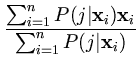
| P(j) = |
(2.21) |
It can be shown that alternating these expectation and maximization steps increases the likelihood L in each iteration step (Bishop, 1995). However, local maxima are not avoided. Further, single isolated data points (outliers) can make the algorithm unstable (Archambeau et al., 2003). If just one pattern is assigned to a unit (that is, the other patterns have almost zero
P(j|![]() )) the variance of the local Gaussian collapses to zero. As an improvement to the local minima problem, annealing schemes (as discussed for the vector quantization, section 2.2) were suggested (Albrecht et al., 2000; Meinicke and Ritter, 2001; Meinicke, 2000). Here, a global variance linked to the width of each Gaussian is gradually reduced during annealing.
)) the variance of the local Gaussian collapses to zero. As an improvement to the local minima problem, annealing schemes (as discussed for the vector quantization, section 2.2) were suggested (Albrecht et al., 2000; Meinicke and Ritter, 2001; Meinicke, 2000). Here, a global variance linked to the width of each Gaussian is gradually reduced during annealing.
The Gaussian mixture model as it is presented here has the disadvantage that all eigenvectors of the local covariance matrix need to be extracted. However, this problem can be overcome if probabilistic PCA is used instead of standard PCA.
 .
. .
.